Color Vision Deficiency Emulation
Overview
Different kinds of limitations can be emulated using the physiologically-based model for simulating color vision deficiency (CVD) of Machado, Oliveira, and Fernandes (2009) deuteranomaly (green cone cells defective), protanomaly (red cone cells defective), and tritanomaly (blue cone cells defective). While most other CVD simulations handle only dichromacy, where one of three cones is non-functional, Machado, Oliveira, and Fernandes (2009) provides a unified model of both dichromacy and anomalous trichromacy, where one cone has shifted spectral sensitivity. As anomalous trichromacy is the most common form of color vision deficiency, it is important to emulate along with the rarer, but more severe dichromacy.
The workhorse function to emulate color vision deficiencies is CVD (not exported) which can take any vector of valid colors and transform them according to a certain CVD transformation matrix and transformation equation. The transformation matrices have been established by Machado, Oliveira, and Fernandes (2009) and are provided by methods of class CVD. The convenience interfaces deutan, protan, tritan, are the high-level functions for simulating the corresponding kind of color blindness with a given severity. A severity of 1 corresponds to dichromacy, 0 to normal color vision, and intermediate values to varying severities of anomalous trichromacy.
For further guidance on color blindness in relation to statistical graphics see Lumley (2013) which accompanies the R package dichromat (Lumley 2013) and is based on earlier emulation techniques Viénot, Brettel, and Mollon (1999).
Illustration: Heatmap with sequential palette
To illustrate that poor color choices can severely reduce the usefulness of a statistical graphic for readers with color vision deficiencies, we employ the infamous RGB rainbow color palette in a heatmap. In base R this can be generated by rainbow(end = 2/3, rev = True)(5) ranging from red (for high values) to blue (for low values).
The poor results for the RGB rainbow palette are contrasted with a proper sequential palette ranging from dark blue to light yellow: sequential_hcl("Blue-Yellow")(5).
The statistical graphic employed for illustration is a heatmap of the well-known Maunga Whau volcano data from base R. This heatmap is easily available as demoplot(x, "Heatmap") where x is the color vector to be used, e.g.,
from colorspace import rainbow, deutan

print(rainbow(end = 2/3, rev = True)(5))
print(deutan(rainbow(end = 2/3, rev = True)(5)))
['#0000FF', '#00FFFF', '#00FF00', '#FFFF00', '#FF0000']
['#003DFB', '#D0DDFF', '#EFD63A', '#FFFA31', '#A39000']and so on. To aid the interpretation of the heatmap a perspective display using only gray shades is included first, providing another intuitive display of what the terrain around Maunga Whau looks like.
import numpy as np
from mpl_toolkits.mplot3d import Axes3D
import matplotlib.pyplot as plt
from matplotlib.colors import LightSource

from colorspace import sequential_hcl, dataset

# Color palette to use (grayscale)
pal  = sequential_hcl(c1 = 0, c2 = 0)

# Loading volcano
data = dataset("volcano")
Y    = np.linspace(1, data.shape[0], data.shape[0])
X    = np.linspace(1, data.shape[1], data.shape[1])
X, Y = np.meshgrid(X, Y)

fig, ax = plt.subplots(subplot_kw ={"projection": "3d"}, figsize = (10, 6))

ax.set_axis_off()
ax.set_box_aspect(aspect = (data.shape[1], data.shape[0], data.shape[0] / 3))
fig.subplots_adjust(left = 0, right = 1, bottom = -.4, top = 1.6)

# Create/calculate facing colors using custom shading
ls      = LightSource(270, 45)
fcolors = ls.shade(data, cmap = pal.cmap(), vert_exag=0.1, blend_mode='soft')

surf = ax.plot_surface(X, Y, data, rstride = 1, cstride = 1, facecolors = fcolors,
                       linewidth = 0, antialiased = False, shade = False)

plt.show()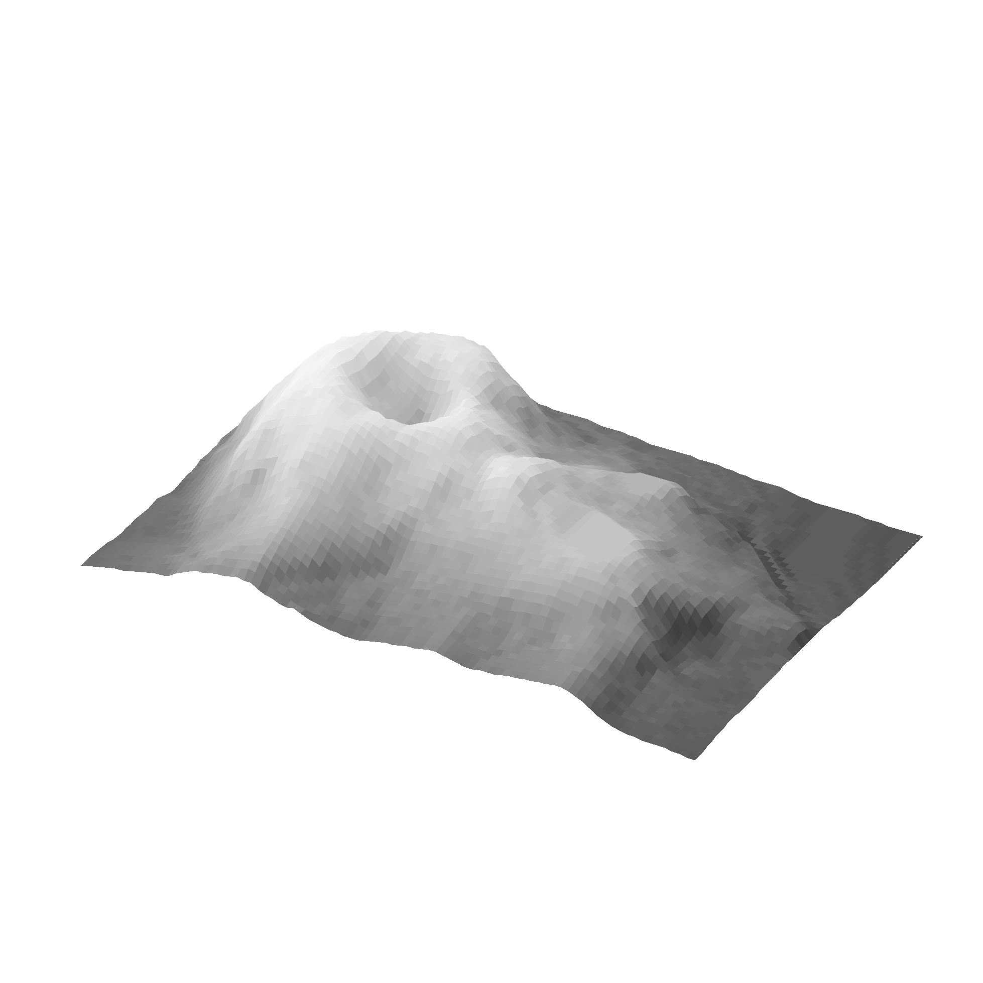
Subsequently, all combinations of palette and color vision deficiency are visualized. Additionally, a grayscale version is created with desaturate.
from matplotlib import pyplot as plt
from colorspace import demoplot, sequential_hcl, rainbow
from colorspace import desaturate, protan, deutan, tritan

# Picking 7 colors from two different color palettes
col_rainbow = rainbow(end = 2/3, rev = True)(7)
col_hcl     = sequential_hcl("Blue-Yellow", rev = True)(7)

fig, axes = plt.subplots(5, 2, figsize = (9, 13))

demoplot(col_rainbow, type_ = "Heatmap", ax = axes[0, 0], ylabel = "Original",
         title = "rainbow(end = 2/3, rev = True)(7)")
demoplot(col_hcl,     type_ = "Heatmap", ax = axes[0, 1], ylabel = "Original",
         title = "sequential_hcl(\"Blue-Yellow\", rev = True)(7)")

demoplot(desaturate(col_rainbow), type_ = "Heatmap", ax = axes[1, 0], ylabel = "Desaturated")
demoplot(desaturate(col_hcl),     type_ = "Heatmap", ax = axes[1, 1], ylabel = "Desaturated")

demoplot(deutan(col_rainbow),     type_ = "Heatmap", ax = axes[2, 0], ylabel = "Deuteranope")
demoplot(deutan(col_hcl),         type_ = "Heatmap", ax = axes[2, 1], ylabel = "Deuteranope")

demoplot(protan(col_rainbow),     type_ = "Heatmap", ax = axes[3, 0], ylabel = "Protanope")
demoplot(protan(col_hcl),         type_ = "Heatmap", ax = axes[3, 1], ylabel = "Protanope")

demoplot(tritan(col_rainbow),     type_ = "Heatmap", ax = axes[4, 0], ylabel = "Tritanope")
demoplot(tritan(col_hcl),         type_ = "Heatmap", ax = axes[4, 1], ylabel = "Tritanope")

plt.show()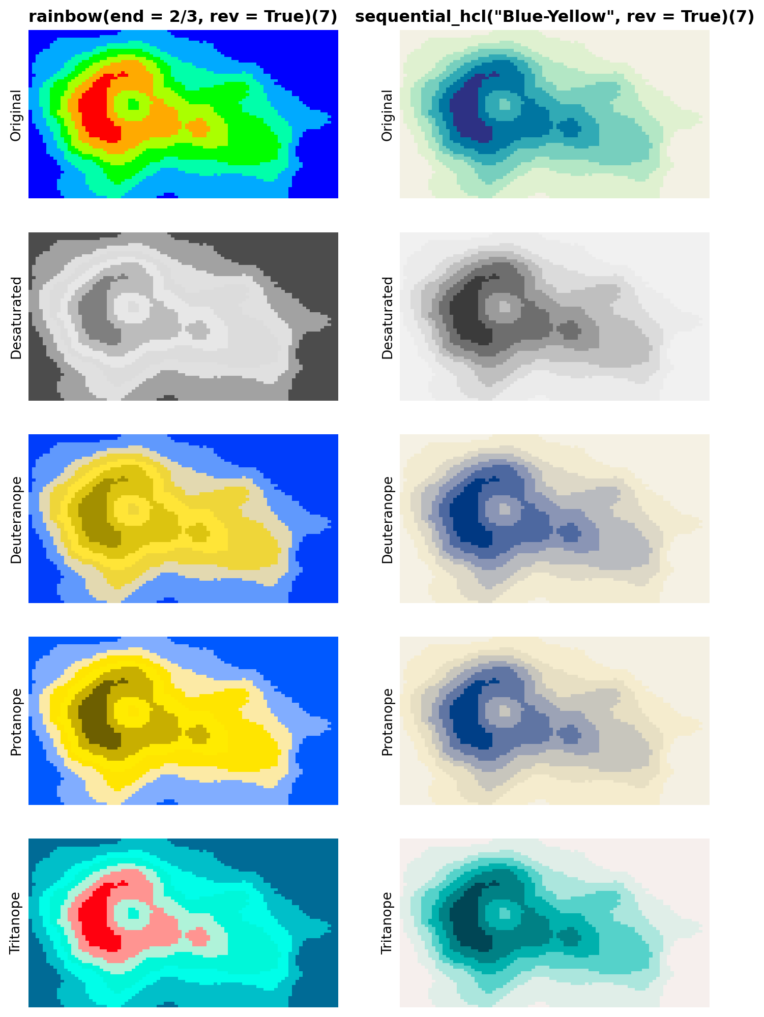
This clearly shows how poorly the RGB rainbow performs, often giving quite misleading impressions of the terrain around Maunga Whau. In contrast, the HCL-based blue-yellow palette works reasonably well in all settings. The most important problem of the RGB rainbow is that it is not monotonic in luminance, making correct interpretation quite hard. Moreover, the red-green contrasts deteriorate substantially in the dichromatic emulations.
Illustration: Map with diverging palette
As another example for the poor performance of the RGB rainbow we employ a shaded map. This is available as demoplot(x, "Map") and is based on county polygons for Alabama, Georgia, and South Carolina along with an artifical variable used for coloring.
Often the red-yellow-green RGB spectrum is used for a diverging palette with yellow as the neutral value. This can easily be generated using rainbow(end = 1/3)(11). However, this palette has again a number of weaknesses, especially that the green-yellow part of the palette almost collapses to the same color when desaturated or when color blindness is emulated.
To illustrate that much more balanced palettes for the same purpose are available the Geyser palette (mimicked from CARTO 2019) is adopted: divergingx_hcl("Geyser"")(11)
from matplotlib import pyplot as plt
from colorspace import demoplot, divergingx_hcl, rainbow
from colorspace import desaturate, protan, deutan, tritan

fig, axes = plt.subplots(5, 2, figsize = (9, 13))

# Picking 11 colors from two different color palettes
col_rainbow = rainbow(end = 1/3)(11)
col_hcl     = divergingx_hcl("Geyser")(11)

demoplot(col_rainbow, type_ = "Map", ax = axes[0, 0], ylabel = "Original",
         title = "rainbow(end = 1/3)(11)")
demoplot(col_hcl,     type_ = "Map", ax = axes[0, 1], ylabel = "Original",
         title = "divergingx_hcl(\"Geyser\")(11)")

demoplot(desaturate(col_rainbow), type_ = "Map", ax = axes[1, 0], ylabel = "Desaturated")
demoplot(desaturate(col_hcl),     type_ = "Map", ax = axes[1, 1], ylabel = "Desaturated")

demoplot(deutan(col_rainbow),     type_ = "Map", ax = axes[2, 0], ylabel = "Deuteranope")
demoplot(deutan(col_hcl),         type_ = "Map", ax = axes[2, 1], ylabel = "Deuteranope")

demoplot(protan(col_rainbow),     type_ = "Map", ax = axes[3, 0], ylabel = "Protanope")
demoplot(protan(col_hcl),         type_ = "Map", ax = axes[3, 1], ylabel = "Protanope")

demoplot(tritan(col_rainbow),     type_ = "Map", ax = axes[4, 0], ylabel = "Tritanope")
demoplot(tritan(col_hcl),         type_ = "Map", ax = axes[4, 1], ylabel = "Tritanope")

plt.show()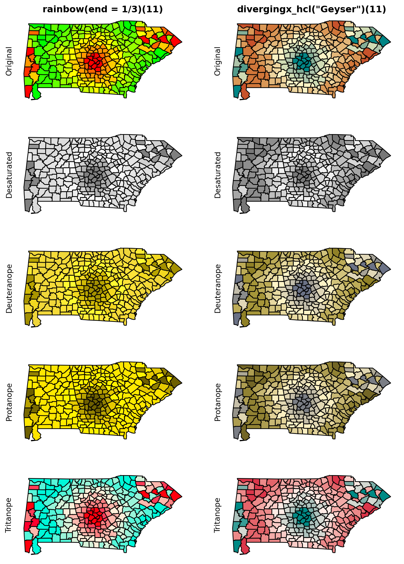
While many versions of the RGB rainbow displays are hard to read because they do not bring out any differences in the green-yellow arm of the palette, the HCL-based palette works reasonably well in all settings. Only the grayscale version cannot bring out the different arms of the palette. However, at least both directions of deviation are visible even if they cannot be distinguished. This is preferable to the RGB rainbow which hides all differences in the green-yellow arm of the palette. (However, if grayscale printing is desired a sequential rather than a diverging palette is probably necessary.)
Manipulating figures
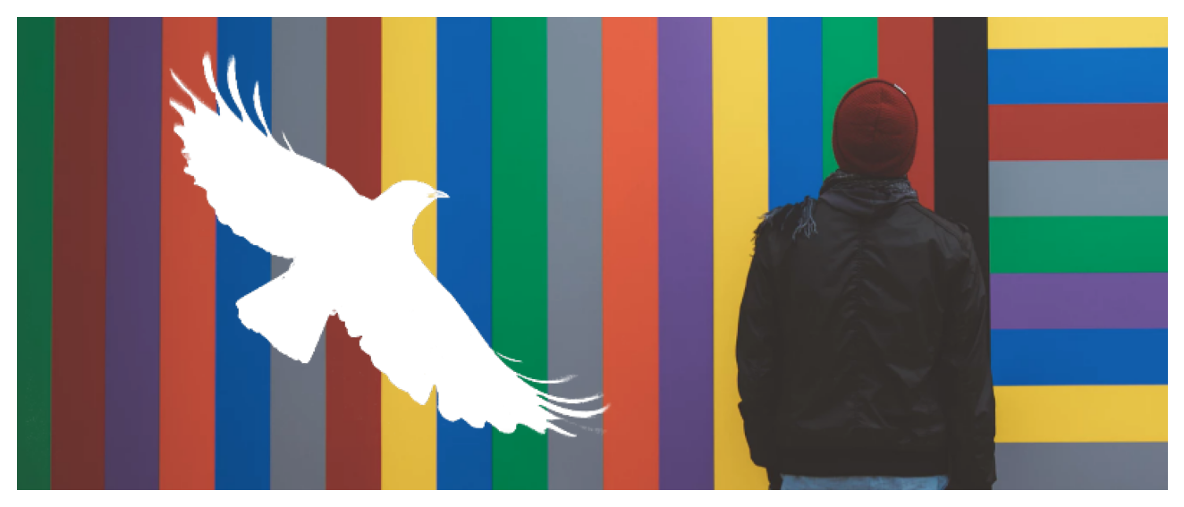
In addition of converting colors and palettes the function cvd_image allows to take an existing pixel image (JPG, PNG) and emulate how people with visual constraints will receive the same picture. This requires imageio to be installed (see Installation).
The first argument of cvd_image can be a path to any pixel image on your local computer OR the string "DEMO". When "DEMO" is used a demo image included in the package will be used (thanks to @mariogogh on unsplash.com; the bird is used to show handling of transparency). The following shows the original (full color) image.
from colorspace import cvd_image
cvd_image("DEMO", "original")
/opt/hostedtoolcache/Python/3.14.2/x64/lib/python3.14/site-packages/colorspace/cvd_image.py:135: UserWarning:
Ignoring specified arguments in this call because figure with num: 1 already exists
cvd_image allows simulate deuteranope, protanope, tritanope, and desaturated versions with different severities (defaults to severity = 1.0). The function reads the RGB(+alpha) coordinates of the pixel image, creates an sRGB object, and calls the requested functions (deutan, protan, tritan, and desaturate) before re-creating the image.
from colorspace import cvd_image
cvd_image("DEMO", ["deutan", "protan", "tritan", "desaturate"])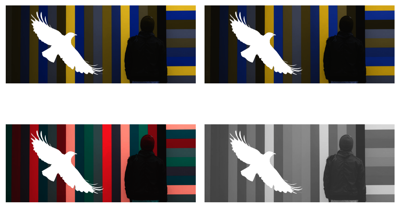
The additional argument output (path to file) can be used to store the result rather than displaying it.