Windrose

The foehnix package comes with methods to create windrose plot for foehn classification models (see getting started, foehnix reference) and observation data. Two types of windrose plots are available:

• density: empirical density
• histogram: empirical circular histogram

Windrose Plot for Observation Data

The windrose function can be called with a set of (observed) wind direction and wind speed values. Wind direction has to be the meteorological wind direction in degrees ([0, 360], 0 and 360 corresponds to wind coming from North, 90 for wind from East, 180 for wind from South, and 270 from West).

# Loading the demo data set for station Ellboegen
data <- demodata("ellboegen")
print(head(data))

##                      dd  ff  rh    t
## 2006-01-01 01:00:00 171 0.6  90 -0.4
## 2006-01-01 02:00:00 268 0.3 100 -1.8
## 2006-01-01 03:00:00 115 5.2  79  0.9
## 2006-01-01 04:00:00 152 2.1  88 -0.6
## 2006-01-01 05:00:00 319 0.7 100 -2.6
## 2006-01-01 06:00:00  36 0.1  99 -1.7

# Plotting windrose
windrose(data$dd, data$ff, type = "density")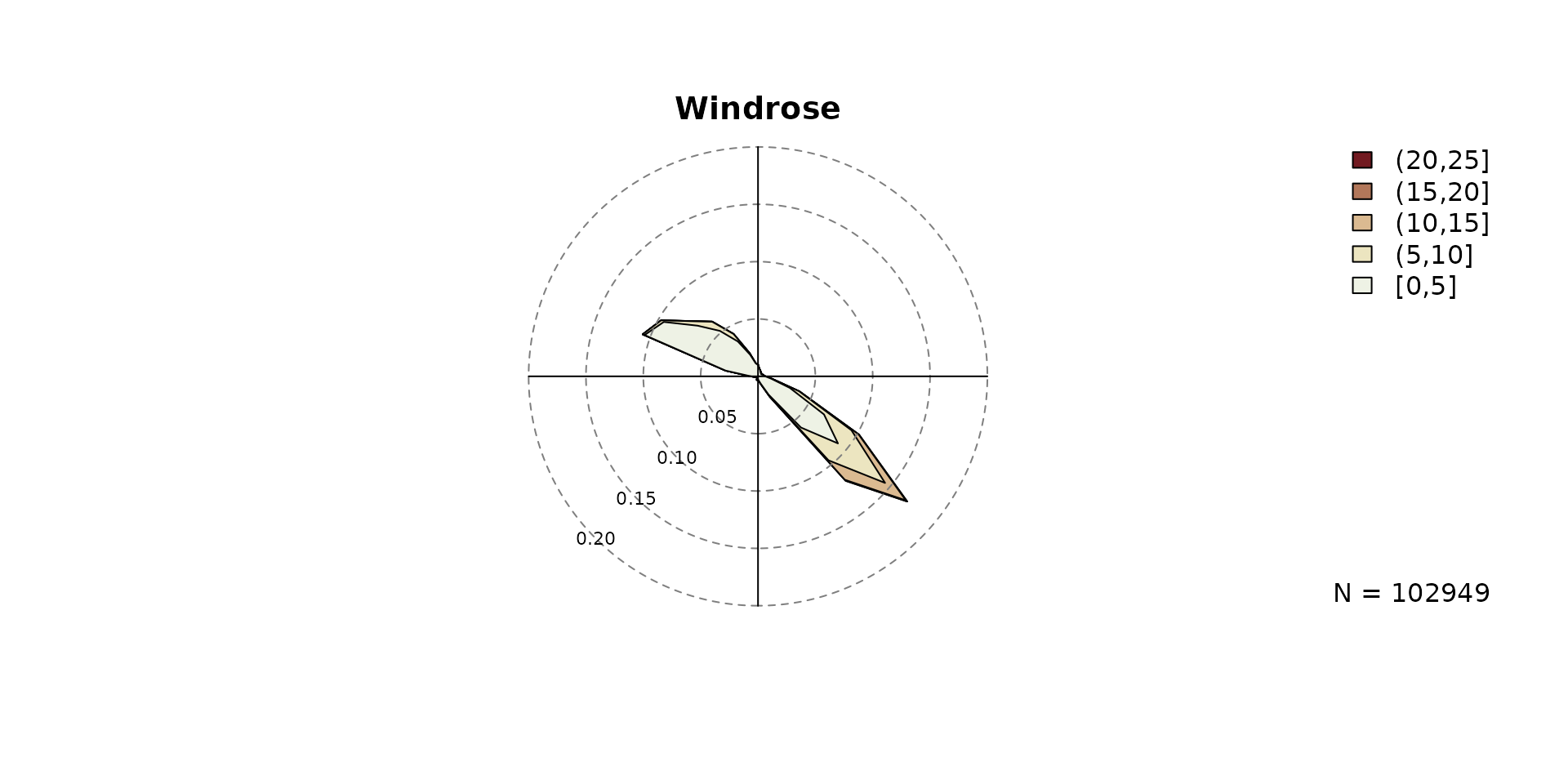

windrose(as.numeric(data$dd), as.numeric(data$ff), type = "histogram")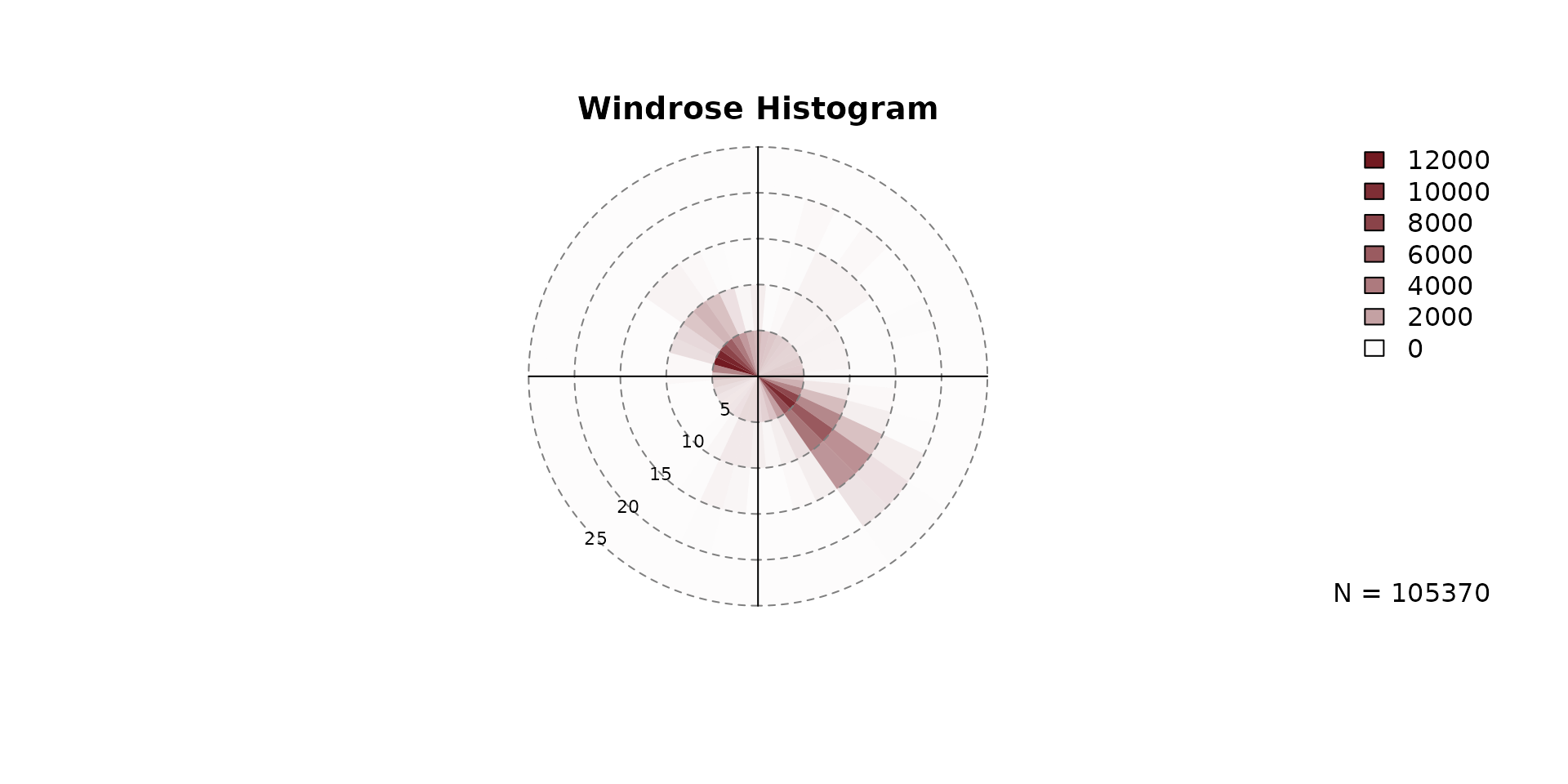

Windrose Plot for foehnix Models

Windrose plots can also be created for foehnix foehn classification models if wind speed and wind direction information has been provided to the foehnix function when estimating the classification model.

# Loading the demo data set for Tyrol (Ellboegen and Innsbruck)
data <- demodata("tyrol") # default
print(head(data))

##                      dd  ff  rh    t crest_dd crest_ff crest_rh crest_t diff_t
## 2006-01-01 01:00:00 171 0.6  90 -0.4      180     10.8      100    -7.8   2.87
## 2006-01-01 02:00:00 268 0.3 100 -1.8      186     12.5      100    -8.0   4.07
## 2006-01-01 03:00:00 115 5.2  79  0.9      181     11.3      100    -7.4   1.97
## 2006-01-01 04:00:00 152 2.1  88 -0.6      178     13.3      100    -7.5   3.37
## 2006-01-01 05:00:00 319 0.7 100 -2.6      176     13.1      100    -7.1   5.77
## 2006-01-01 06:00:00  36 0.1  99 -1.7      184     10.0      100    -6.9   5.07

# Estimate a foehnix classification model
filter <- list(dd = c(43, 223), crest_dd = c(90, 270))
mod <- foehnix(diff_t ~ ff + rh, data = data, filter = filter,
               switch = TRUE, verbose = FALSE)

# Plotting windroses
windrose(mod)

By default, windrose expects that the parameters are called dd (wind direction) and ff (wind speed), however, custom names can also be used.

# Loading the demo data set for station Ellboegen and Sattelberg (combined)
data <- demodata("tyrol") # default
names(data) <- gsub("dd$", "winddir", names(data))
names(data) <- gsub("ff$", "windspd", names(data))
print(head(data))

##                     winddir windspd  rh    t crest_winddir crest_windspd
## 2006-01-01 01:00:00     171     0.6  90 -0.4           180          10.8
## 2006-01-01 02:00:00     268     0.3 100 -1.8           186          12.5
## 2006-01-01 03:00:00     115     5.2  79  0.9           181          11.3
## 2006-01-01 04:00:00     152     2.1  88 -0.6           178          13.3
## 2006-01-01 05:00:00     319     0.7 100 -2.6           176          13.1
## 2006-01-01 06:00:00      36     0.1  99 -1.7           184          10.0
##                     crest_rh crest_t diff_t
## 2006-01-01 01:00:00      100    -7.8   2.87
## 2006-01-01 02:00:00      100    -8.0   4.07
## 2006-01-01 03:00:00      100    -7.4   1.97
## 2006-01-01 04:00:00      100    -7.5   3.37
## 2006-01-01 05:00:00      100    -7.1   5.77
## 2006-01-01 06:00:00      100    -6.9   5.07

# Estimate a foehnix classification model
filter <- list(winddir = c(43, 223), crest_winddir = c(90, 270))
mod <- foehnix(diff_t ~ windspd + rh, data = data, filter = filter,
               switch = TRUE, verbose = FALSE)

# Plotting windroses
windrose(mod, ddvar = "winddir", ffvar = "windspd")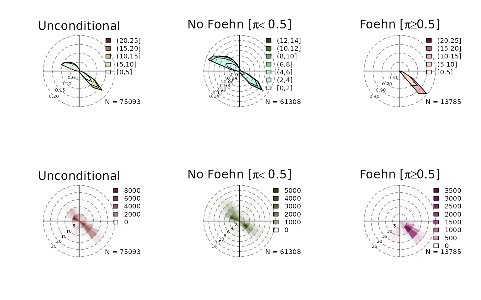

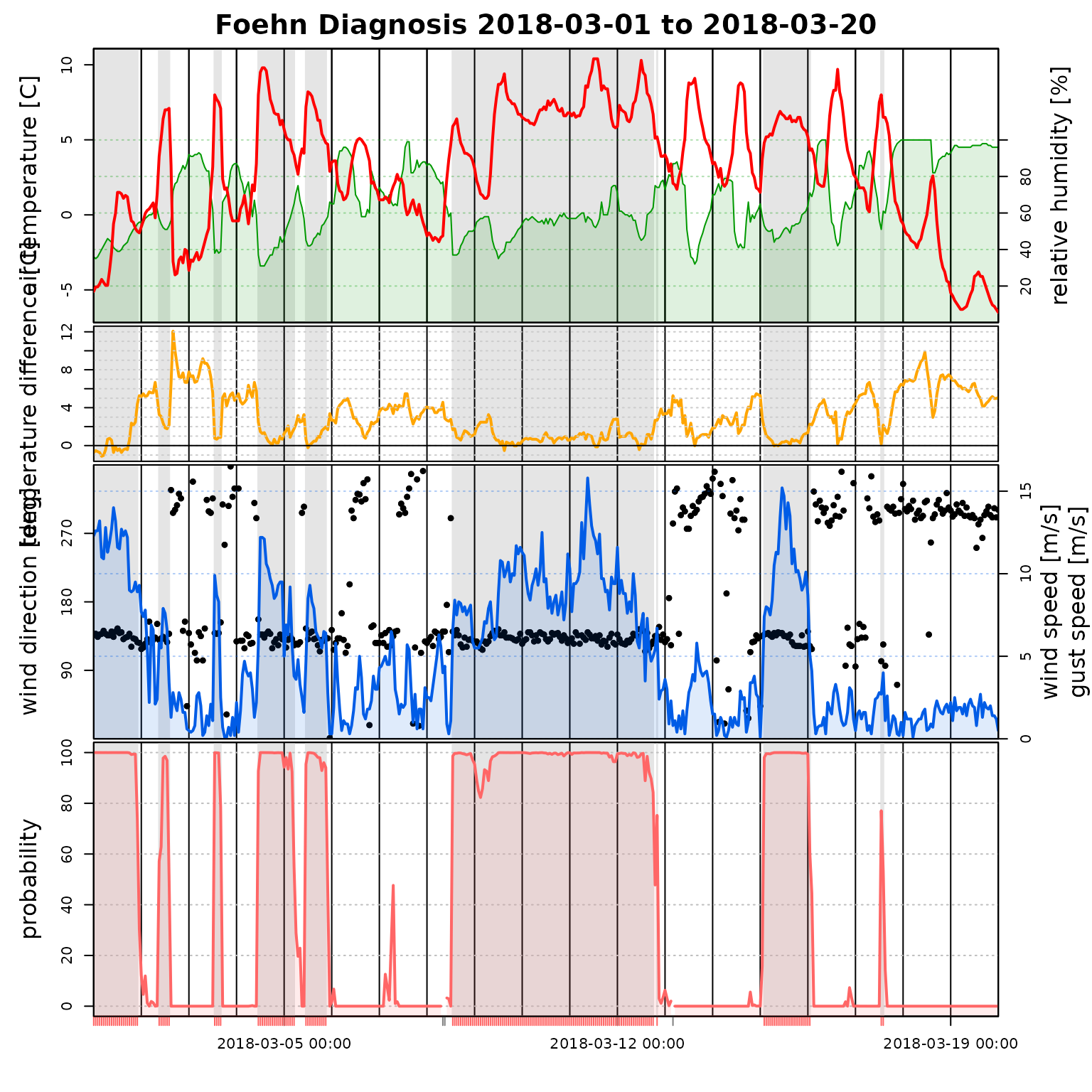
Default Time Series Plot

TODO: Write vignette.

# Loading the demo data set for station Ellboegen and Sattelberg (combined)
data <- demodata("tyrol")
filter <- list(dd = c(43, 223), crest_dd = c(90, 270))
mod <- foehnix(diff_t ~ ff + rh, data = data, filter = filter,
               switch = TRUE, verbose = FALSE)

# Time Series Plot
tsplot(mod, start = "2018-03-01", end = "2018-03-20")