Source:
vignettes/advanced_simulation.Rmd
advanced_simulation.RmdSimulation
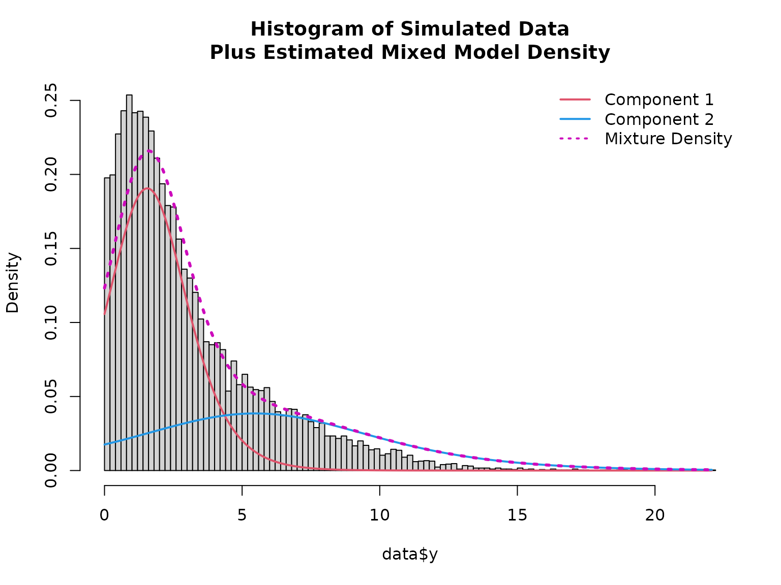
Simulation of two-component mixed distributions without concomitaunt information to test the algorithm.
Left Censored Gaussian
## Loading required package: testthat##
## Attaching package: 'foehnix'## The following object is masked from 'package:utils':
##
## write.csv
# The true parameters of the distribution
true <- list(mu = c(1, 5), sigma = c(1, 2))

# Simulate data based on Gaussian distribution
family <- foehnix:::foehnix_cgaussian(left = 0)
set.seed(666)
data <- data.frame(y = family$r(c(10000, 5000), mu = true$mu, sigma = true$sigma))
data <- zoo(data, as.Date(1:nrow(data), origin = "1970-01-01"))

# Estimate foehnix model
mod <- foehnix(y ~ 1, data = data, left = 0, verbose = FALSE)
## Warning in foehnix(y ~ 1, data = data, left = 0, verbose = FALSE): The EM
## algorithm stopped after one iteration! The coefficients returned are the
## initial coefficients. Indicates that the model as specified is not suitable for
## the data. Suggestion: check model (e.g, using plot(...) and summary(...,
## detailed = TRUE)) and try a different model specification (change formula).
coef(mod)## Coefficients of foehnix model
## Model formula: y ~ 1
## foehnix family of class: censored Gaussian
## Censoring thresholds: left = 0, right = Inf
## No concomitant model in use
##
## Coefficients
## mu1 sigma1 mu2 sigma2
## 0.9745221 0.9518903 4.8901478 1.9873473
# Path of log-likelihood sum during optimization
plot(mod, which = "loglik")
# Plotting mixed distribution
# Calculate density of the two components
x <- seq(min(data$y), max(data$y), length = 501)
density1 <- family$d(x, coef(mod)["mu1"], coef(mod)["sigma1"])
density2 <- family$d(x, coef(mod)["mu2"], coef(mod)["sigma2"])
hist(data$y, breaks = 100, freq = FALSE,
     main = "Histogram of Simulated Data\nPlus Estimated Mixed Model Density")
lines(x, density1 * (1 - mean(fitted(mod))), col = 2, lwd = 2)
lines(x, density2 * mean(fitted(mod)),       col = 4, lwd = 2)
lines(x, density1 * (1 - mean(fitted(mod))) + density2 * mean(fitted(mod)), col = 6, lty = 3, lwd = 3)
legend("topright", col = c(2, 4, 6), lwd = 2, lty = c(1, 1, 3), bty = "n",
       legend = c("Component 1", "Component 2", "Mixture Density"))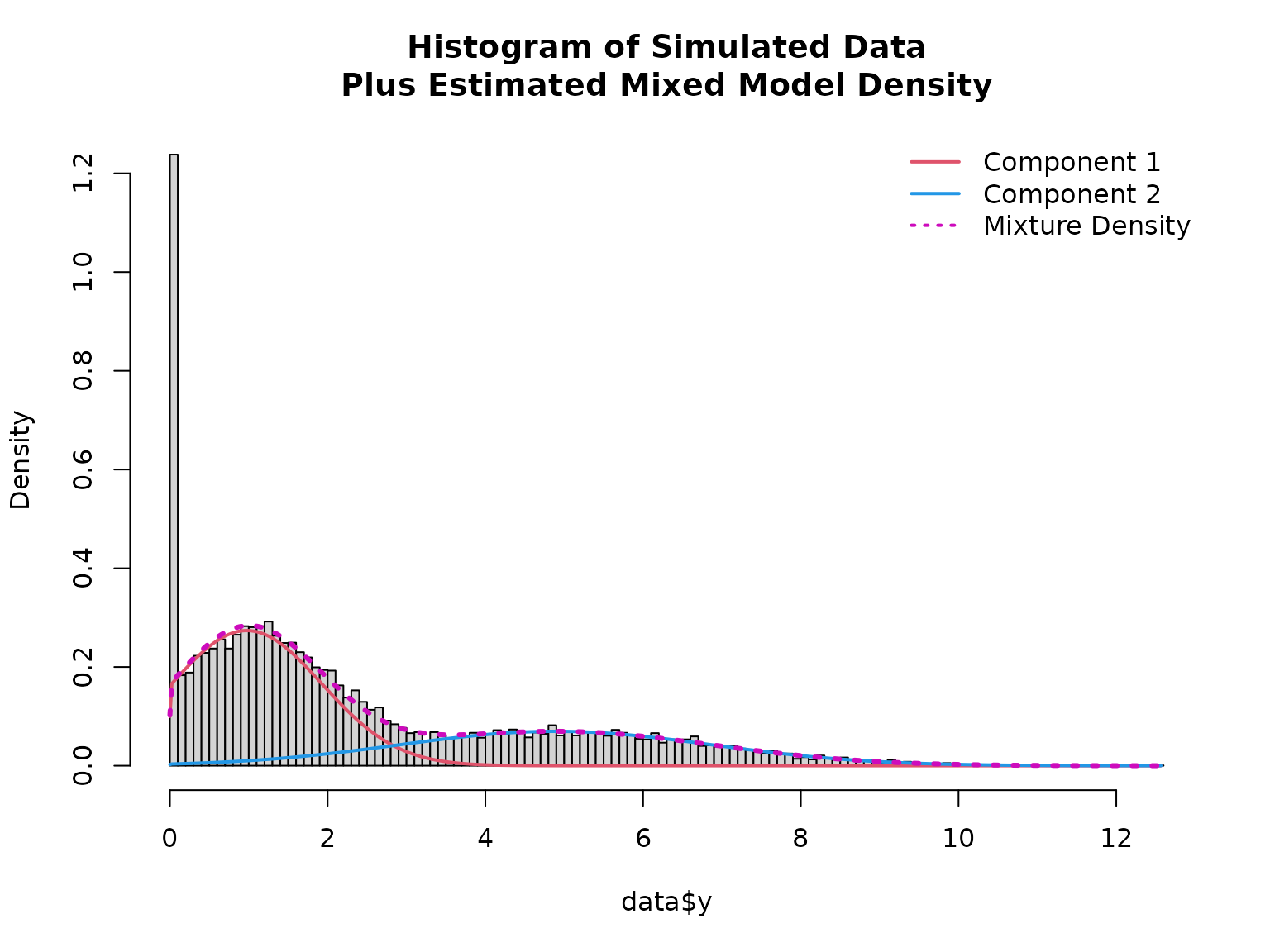
Left Truncated Gaussian
library("foehnix")
# The true parameters of the distribution
true <- list(mu = c(1, 5), sigma = c(1, 2))

# Simulate data based on Gaussian distribution
family <- foehnix:::foehnix_tgaussian(left = 0)
set.seed(666)
data <- data.frame(y = family$r(c(10000, 5000), mu = true$mu, sigma = true$sigma))
data <- zoo(data, as.Date(1:nrow(data), origin = "1970-01-01"))

# Estimate foehnix model
mod <- foehnix(y ~ 1, data = data, left = 0, verbose = FALSE, tol = -Inf)
coef(mod)
## Coefficients of foehnix model
## Model formula: y ~ 1
## foehnix family of class: censored Gaussian
## Censoring thresholds: left = 0, right = Inf
## No concomitant model in use
##
## Coefficients
## mu1 sigma1 mu2 sigma2
## 1.2322662 0.7178724 4.8240012 2.0164347
# Path of log-likelihood sum during optimization
plot(mod, which = "loglik")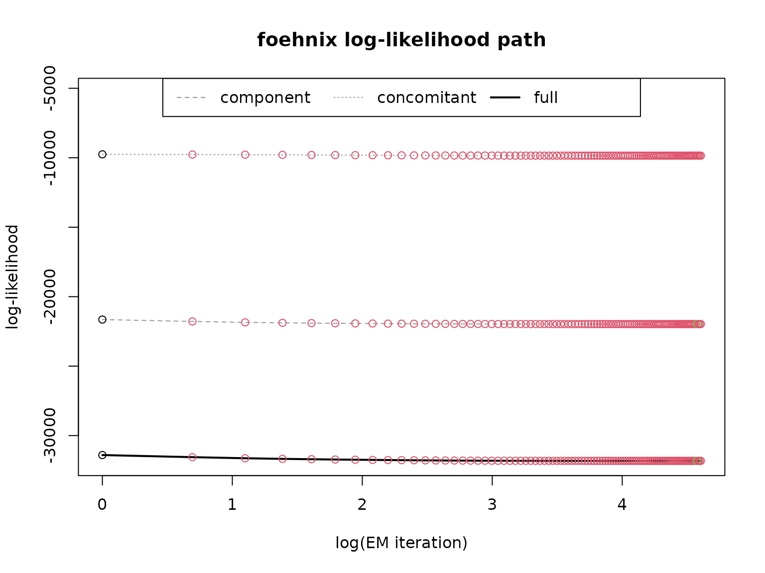
# Plotting mixed distribution
# Calculate density of the two components
x <- seq(min(data$y), max(data$y), length = 501)
density1 <- family$d(x, coef(mod)["mu1"], coef(mod)["sigma1"])
density2 <- family$d(x, coef(mod)["mu2"], coef(mod)["sigma2"])
hist(data$y, breaks = 100, freq = FALSE,
     main = "Histogram of Simulated Data\nPlus Estimated Mixed Model Density")
lines(x, density1 * (1 - mean(fitted(mod))), col = 2, lwd = 2)
lines(x, density2 * mean(fitted(mod)),          col = 4, lwd = 2)
lines(x, density1 * (1 - mean(fitted(mod))) + density2 * mean(fitted(mod)), col = 6, lty = 3, lwd = 3)
legend("topright", col = c(2, 4, 6), lwd = 2, lty = c(1, 1, 3), bty = "n",
       legend = c("Component 1", "Component 2", "Mixture Density"))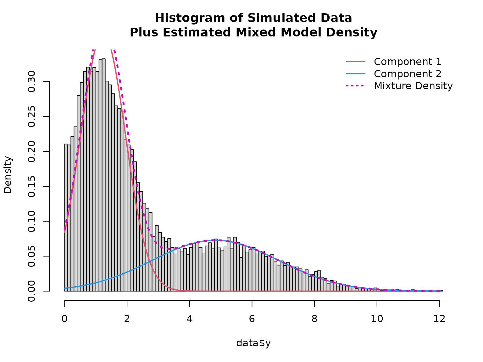
Left Censored Logistic
library("foehnix")
# The true parameters of the distribution
true <- list(mu = c(1, 5), sigma = c(1, 2))

# Simulate data based on logistic distribution
family <- foehnix:::foehnix_clogistic(left = 0)
set.seed(666)
data <- data.frame(y = family$r(c(10000, 5000), mu = true$mu, sigma = true$sigma))
data <- zoo(data, as.Date(1:nrow(data), origin = "1970-01-01"))

# Estimate foehnix model
mod <- foehnix(y ~ 1, data = data, left = 0, verbose = FALSE)
## Warning in foehnix(y ~ 1, data = data, left = 0, verbose = FALSE): The EM
## algorithm stopped after one iteration! The coefficients returned are the
## initial coefficients. Indicates that the model as specified is not suitable for
## the data. Suggestion: check model (e.g, using plot(...) and summary(...,
## detailed = TRUE)) and try a different model specification (change formula).
coef(mod)## Coefficients of foehnix model
## Model formula: y ~ 1
## foehnix family of class: censored Gaussian
## Censoring thresholds: left = 0, right = Inf
## No concomitant model in use
##
## Coefficients
## mu1 sigma1 mu2 sigma2
## 0.7618013 1.4161469 5.1480930 3.0871087
# Path of log-likelihood sum during optimization
plot(mod, which = "loglik")
# Plotting mixed distribution
# Calculate density of the two components
x <- seq(min(data$y), max(data$y), length = 501)
density1 <- family$d(x, coef(mod)["mu1"], coef(mod)["sigma1"])
density2 <- family$d(x, coef(mod)["mu2"], coef(mod)["sigma2"])
hist(data$y, breaks = 100, freq = FALSE,
     main = "Histogram of Simulated Data\nPlus Estimated Mixed Model Density")
lines(x, density1 * (1 - mean(fitted(mod))), col = 2, lwd = 2)
lines(x, density2 * mean(fitted(mod)),       col = 4, lwd = 2)
lines(x, density1 * (1 - mean(fitted(mod))) + density2 * mean(fitted(mod)), col = 6, lty = 3, lwd = 3)
legend("topright", col = c(2, 4, 6), lwd = 2, lty = c(1, 1, 3), bty = "n",
       legend = c("Component 1", "Component 2", "Mixture Density"))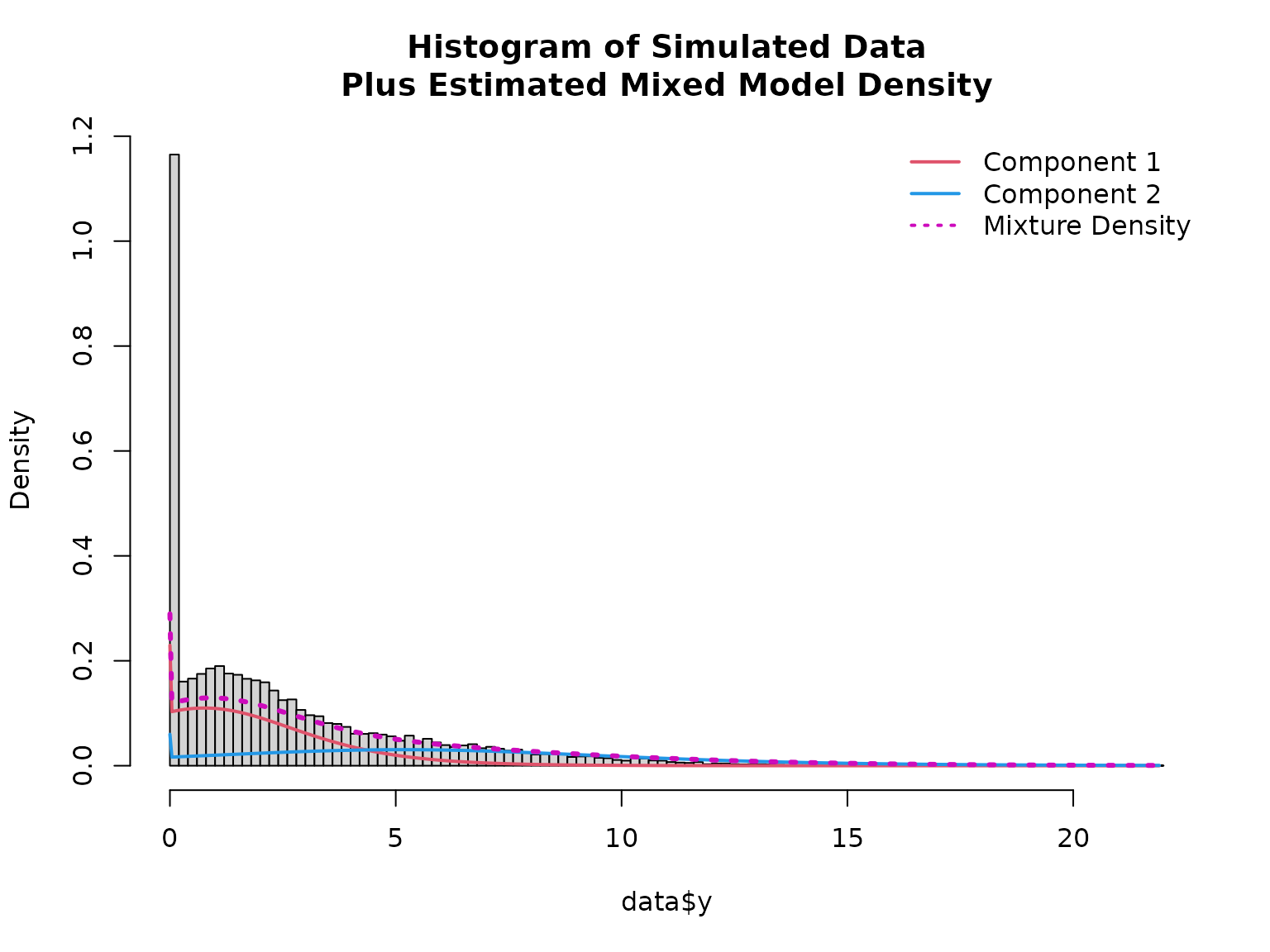
Left Truncated Logistic
library("foehnix")
# The true parameters of the distribution
true <- list(mu = c(1, 5), sigma = c(1, 2))

# Simulate data based on logistic distribution
family <- foehnix:::foehnix_tlogistic(left = 0)
set.seed(666)
data <- data.frame(y = family$r(c(10000, 5000), mu = true$mu, sigma = true$sigma))
data <- zoo(data, as.Date(1:nrow(data), origin = "1970-01-01"))

# Estimate foehnix model
mod <- foehnix(y ~ 1, data = data, left = 0, verbose = FALSE, tol = -Inf)
coef(mod)
## Coefficients of foehnix model
## Model formula: y ~ 1
## foehnix family of class: censored Gaussian
## Censoring thresholds: left = 0, right = Inf
## No concomitant model in use
##
## Coefficients
## mu1 sigma1 mu2 sigma2
## 1.5543862 0.9642826 5.4678146 2.8892143
# Path of log-likelihood sum during optimization
plot(mod, which = "loglik")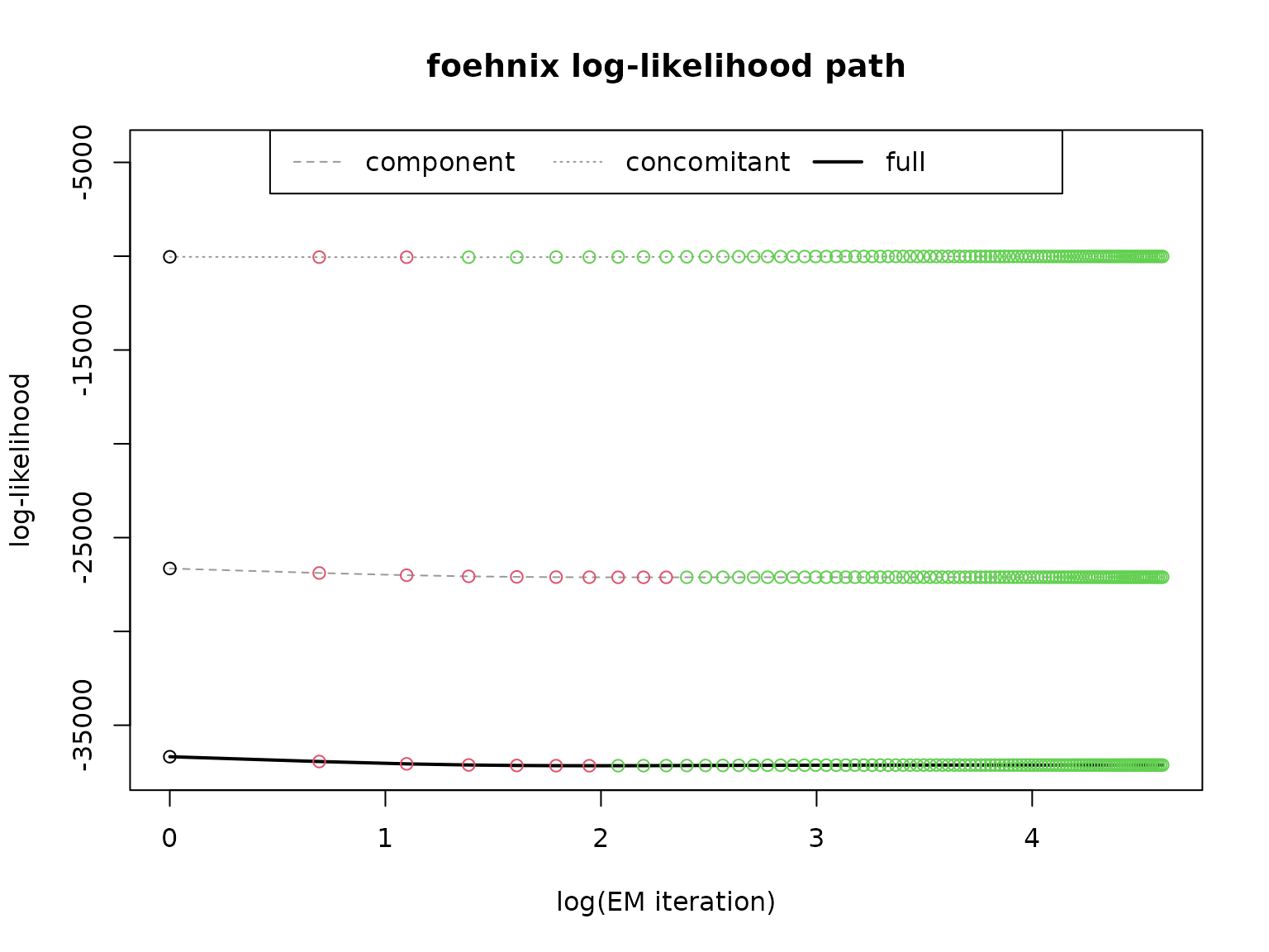
# Plotting mixed distribution
# Calculate density of the two components
x <- seq(min(data$y), max(data$y), length = 501)
density1 <- family$d(x, coef(mod)["mu1"], coef(mod)["sigma1"])
density2 <- family$d(x, coef(mod)["mu2"], coef(mod)["sigma2"])
hist(data$y, breaks = 100, freq = FALSE,
     main = "Histogram of Simulated Data\nPlus Estimated Mixed Model Density")
lines(x, density1 * (1 - mean(fitted(mod))), col = 2, lwd = 2)
lines(x, density2 * mean(fitted(mod)),       col = 4, lwd = 2)
lines(x, density1 * (1 - mean(fitted(mod))) + density2 * mean(fitted(mod)), col = 6, lty = 3, lwd = 3)
legend("topright", col = c(2, 4, 6), lwd = 2, lty = c(1, 1, 3), bty = "n",
       legend = c("Component 1", "Component 2", "Mixture Density"))